Aggregation in OBIEE

OBIEE as a reporting tool provides tremendous capabilities to do analytical reporting. Many new functions and decision features helps any user to do different reporting using OBIEE. For any analytical reporting anyone would accept that aggregation is the most basic and important tool. And so OBIEE provides amazing capabilities for doing different types of aggregation.

In this article we would see places where OBIEE provides features and capability is apply aggregation rules.

1.       The first and the most basic is the Aggregation tab in logical column of any logical table in BMM layer of RPD. In the figure below the area highlighted in red is used to set the default aggregation rule for any logical table column.

2.       The aggregation tab is used to specify default aggregation rules that would get applied when any user tries to query this column with other dimensions. OBIEE also provides a feature to specify different aggregation rules to be applied for different dimension table. To use this feature, one needs to check the “Based on dimensions” option as highlighted in green in above figure and specify different aggregation formula for different dimension.

If nothing is specified for any dimension then the aggregation rule as specified in the “Other” section gets applied in the physical query.

3.       The second feature that OBIEE provides related to aggregation is the concept of level based measure in any fact table. A level based measure in OBIEE is a measure in any fact table that is always pinned to a certain level of dimension table. Suppose there is a requirement where you have to show the monthly as well as yearly sales of products as two columns of a report. To do this one has to sum up sales column on monthly as well as yearly basis. To achieve this is SQL, you have to fire two queries and then join them together to get the final result.

SELECT time.cal_year,

        time.cal_period,

        SUM(sales.amount)

FROM sales,

       Time

WHERE sales.time_id=time.time_id

GROUP BY time.cal_year,

       time.cal_period;

And,

SELECT time.cal_year,

        SUM(sales.amount)

FROM sales,

       Time

WHERE sales.time_id=time.time_id

GROUP BY time.cal_year;

And then join the two result sets based on the cal_year column to get the monthly as well as yearly sales figure. However in OBIEE one can achieve this only when we tell OBIEE that one of the measure needs to be calculated at year level and one at monthly level separately and then it has to stitch the tow result sets together to get the final result. This can be done in OBIEE by creating a level based measure which is pinned at year level of time dimension hierarchy.

As before, we would consider a typical sales demo model. Here we would create a logical column amount_year in sales logical table and map it to sames.amount column and set the default aggregation rule as SUM as specified in step 2. Then we would double click on the sales.amount_year column in the BMM layer and go to Levels tab. This tab would be used to define the level of this measure.

As we have to pin the measure only related to Time_DDim, So we would specify the level for Time dimension as year level.

Now when a user queries columns as time.cal_year, time.cal_month, sales.amount and sales.amount_year column in OBIEE, the report produced would provide yearly as well as monthly sum of sales. Here one thing to mention is that if no level is specified for any dimension in the levels tab then it is considered as detail level for remaining dimensions. In the above example for location and product dimension the level pinned with amount_year column is detail level.

One of the most important and intriguing concept in OBIEE related to aggregation concept is the feature of aggregate navigation and fragmentation. In the next blog we would explore the concept of aggregate navigation.

Repository and Session variable in OBIEE

There has been a lot of discussion on the ETL aspect of business intelligence solution. Let us now discuss about the reporting aspect of business intelligence. Oracle BI as a part of fusion middleware solution provide its standard reporting platform Oracle business intelligence enterprise edition(OBIEE 11g) for doing reporting. OBIEE 11g as a reporting tool provides feature and functionalities that are used to provide out of box solution to different business needs. It leverages the weblogic technology and legacy Siebel Analytics solution platform.

In OBIEE 11g we have a concept of variables. Variables in OBIEE are used to store global values that are used in multiple areas. There are two types of variables in OBIEE.

1. Repository variable: These variables are initialized only once or are refreshed only after a certain interval. These variables are used for storing values like global currency for reporting. Default values for all the users for some variable.
These variables are of two types:
   a. Static variable: These variables are initialized during creation time only and the values can be modified only from       repository administration tool > Variable Manager.
   b. Dynamic variable: These variable can be changed after creation using event polling.

2. Session variable: These variables have a copy for each user instance. These variables are initialized after a user logs in to the system.

The variable are initialized using the initialization block. These variables are of two types.
   a. System variable: These variables are system sepcific variable like USER etc. These are system reserved variables and no new variables can be defined with the same name as system variable.
   b. Non System variable: These variables are defined by user for project spefic purpose and are initialized using initialization block at each login by any user.

Although you would think why I suddenly started with variables in OBIEE as a start of discussion on OBIEE. Well this has to do with the problem I faced while learning OBIEE. During my learning curve I had a lot of confusion regarding variables and its types in OBIEE. In a hope to solve my problem I endlessly searched for a place to clear my concept. However all my endeavours ended in failure.

In the next post we would discuss about the concept of aggregation in BMM layer of OBI.

OPB backend query to get names of mapping with a table as lookup source

select DISTINCT opb_subject.subj_name "Folder Name"
,opb_mapping.mapping_name "Mapping Name"
from
opb_widget_inst,
opb_widget_attr,
opb_mapping,
opb_subject
where opb_widget_inst.widget_type=11
and opb_widget_attr.attr_id=2
and opb_widget_inst.widget_id=opb_widget_attr.widget_id
and opb_mapping.mapping_id=opb_widget_inst.mapping_id
and opb_mapping.subject_id=opb_subject.subj_id
and UPPER(attr_value) like '%<<Source Name>>%';

Oracle application security using Oracle's Row level security

As more and more application are being developed to support enterprise needs, security is becoming more and more demanding subject for research and innovation. Oracle's DBMS_RLS in collaboration with Application Context can be used for implementing fine grained access security. In this article we will see the step by step process to implement fine grained access using DBMS_RLS package.

DBMS_RLS package is used to add a dynamic predicate based on user's environment attributes set in its application context.
An application context enables application developers to create, set and access application attributes by acting as a lookup storage from where user's environment attributes can be accessed. Oracle has predefined application context, USERENV which can also be used for this purpose.

Here we will see steps to create custom application context for meeting requirements that cannot be fulfilled using USERENV application context.

Consider an application which has an employee table and orders table in OE schema. Employee table stores all the employee imformation along with the ORG_ID which points to the organisation in which the employee works in. We need to implement a RLS on orders table which allows and employee to see only those orders which are being ordered from their organization. Orders table also has a column called BILL_FROM_ORG_ID which stores the organization from which the order has been placed.

To create an application context ORD_SEC we need to create a package which can be used to set the attributes of the context. This package is called the trusted package.

1) Create a trusted package.

CREATE OR REPLACE PACKAGE app_security
IS
    PROCEDURE set_context_attribute;
END app_security;

CREATE OR REPLACE PACKAGE BODY app_security
IS
    PROCEDURE set_context_attribute IS
        v_org_id NUMBER;
    BEGIN
        SELECT ORG_ID INTO v_org_id from employee where emp_name=SYS_CONTEXT('USERENV','SESSION_USER');
        DBMS_SESSION.SET_CONTEXT('ORD_SEC','ORG_ID',v_org_id);
    END set_context_attribute;

END app_security;

2) After creation of the trusted package we need to create application context ORD_SEC which should be connected to the package app_security.

CREATE CONTEXT ORD_SEC USING app_security;

3) Now we need to create a logon trigger that should invoke the trusted package procedure app_security.set_context_attribute to set the attribute in the context so that it can be used by the application for further processing and security implementation.

4) Now when the custom application context has been created which sets the custom context attributes when ever user logs in to the database, we need to create a security policy package that will return the predicate to be used with statements assigned in the policy.

CREATE OR REPLACE PACKAGE sec_policy IS
FUNCTION get_policy_predicate RETURN VARCHAR2;
END sec_policy;

CREATE OR REPLACE PACKAGE BODY IS

FUNCTION get_policy_predicate RETURN VARCHAR2
v_org_id number;
v_predicate VARCHAR2(200);
IS
v_predicate:='BILL_TO_ORG_ID='||SYS_CONTEXT('ORD_SEC','ORG_ID');
RETURN v_predicate;

END get_policy_predicate;


5) After the creation of policy function, we need to create a policy that is used to add predicate to any database object.For this purpose we use DBMS_RLS predefined package.

EXEC DBMS_RLS.ADD_POLICY('OE','ORDERS','ORD_POLICY','SYS','SEC_POLICY.GET_POLICY_PREDICATE','SELECT');

The statement adds a policy ORD_POLICY to ORDERS table in OE schema using package procedure SEC_POLICY.GET_POLICY_PREDICATE in SYS schema for select statements.

Now whenever a user queries table ORDERS as,

SELECT * FROM ORDERS;

Then Oracle server will add the predicate WHERE BILL_TO_ORG_ID=<<The organization ID of the user>>.

You can try creating more complex security using DBMS_RLS package.  

Informatica Treat Source Rows Option

In Informatica session you would have noticed an option in properties tab, Treat Source Rows as. This option effects how informatica treats rows being processed. The options available for this are 'Insert', 'Update', 'Delete', 'Data Driven'. Selecting any option effects
the way rows are processed. But for some case viz, Update and Data Driven Individual Target table option also contributes to way rows are processed. Here, we will see the effect of options being selected.

Treat Source Rows as - Insert

Individual Target option: Selecting insert option will insert rows. Disabling this option will lead to rejection of records irrespective of what other options (delete, update as update, update as insert, update else insert) are selected.

Treat Source Rows as - Delete

Individual Target option: Selecting delete option will delete the rows. Disabling this option will lead to rejection of records irrespective of what other options (insert, update as update, update as insert, update else insert) are selected.

Treat Source Rows as - Update

Individual Target option:

insert: If this is selected, Integration service uses Target update option. If disabled Integration service rejects all rows if Update as Insert or Update else Insert is selected.

update as update: Integration service updates all rows irrespective of any other target option.

update as insert: Integration service inserts all rows marked for update if the insert option is also selected else rows are rejected.

update else insert: Integration service updates existing rows and inserts new rows given the insert option is also selected.

delete: Integration service ignores this option.

Processing performed by Integration service are represented in tabular form:

DTM Buffer

DTM buffer is a temporary storage area for storing temporary data for caching data used by transformation.  Buffer is divided into blocks. The buffer size and block size for a session is tunable.

We can find out number of blocks using formula,

(Number of Blocks)=0.9*((DTM Buffer Size) / (Buffer Block Size))

Slow Reader, Writer or Transformation thread can be an indication requirement for DTM buffer tuning.

                 

    Tuning the DTM buffer:               

§  Buffer block size:

·         At least  100 rows/block is recommended.

·         Block size should be calculated by taking the maximum size for a row.

·         Number of blocks can then be calculated using the formula.

§  Buffer size should be increased by multiple of blocks.

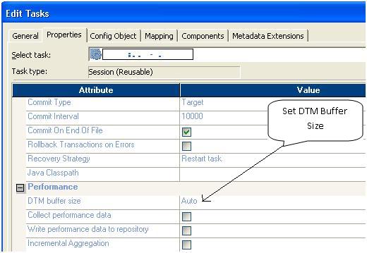
DTM buffer size configuration in an Informatica session:

 

Configure DTM buffer block size:

To utilize the increased DTM buffer, we should also increase the commit interval to some large value to reduce the number of writes to the database.

Build an Informatica mapping: A step by step guide

Building a sample map in informatica is not a very difficult task.You just need is a basic knowledge about informatica client tools and what a mapping should consist of.


Prerequisites to build an informatica mapping:

• An informatica server installed and set up on a server machine.

• An informatica repository created.

• Informatica client tools i.e. Powercenter Mapping Designer, Powercenter Workflow Manager, Powercenter Workflow Monitor installed on client machine.

The first and the foremost task for developing a mapping in informatica powercenter is to open the designer tools. You can find the tool with following icon in All programs under Start Menu:

After starting the designer, you need to add a Domain where informatica repository is located. This is done so that all the development work is saved to that repository.

To add a domain in informatica client:

1. In informatica designer, click on Repository option in the menu and select Configure Domain.
   
   
   
    
2. Click on the small box shown in red to add a new domain.
   
   
   
   
   
    
   
3. Feed in the host/port details of the domain gateway node of informatica server. As informatica has a feature of load balancing. So, there can be more than one server node. But a client can connect to only one node on the server, which is called the gateway node.
   
   
   
   
   
   
4.  After this a repository is added to the client. All the work done can now be saved in the repository. You will be able to see a repository in the left pane in the designer client
5. Right click or double click on the repository and feed in the username/password of the repository as set during repository setup.
   
   
   
    
6.    As a mapping in informatica is an ETL process used to extract data from source and load that data after transforming the data by applying some process to the target. So for building a basic mapping one needs at least one source, one target and in between a transformation process.
7.      For a source in informatica we have source definition i.e. the structure of the source. The columns in the source definition or target definition are called ports in informatica.

To create or import a source definition in informatica:

    1. In the Designer, click Tools > Source Analyzer to open the Source Analyze.

     2. Double-click the Sample folder to view its contents.

    3. Every folder contains nodes for sources, targets, schemas, mappings, mapplets, cubes,  dimensions and reusable transformations.

    4.Click Sources from the menu in the designer > Import from Database.

    5.  Select the ODBC data source to access the database containing the source tables. (To import you have to define an ODBC source in the system (From Control Panel>Administrative tool>Data sources.)

              To define an ODBC data source:

                       · Go to Control Panel>Administrative tool>Data sources

                              · Click on System DSN

                              · Click Add

                     · Select the driver used to connect to the database(Usually Microsoft wire protocol driver from Oracle in case database is oracle)

                              · Give the necessary credentials like host/port/username/password of database server.

                             · Click Ok to create an ODBC Source

    3. Enter the user name and password to connect to this database. Also, enter the name of the source table owner, if necessary.(In Oracle, the owner name is the same as the user name).

    4. Click Connect.

    5. In the Select tables list, expand the TABLES heading

    6. Select the tables from the list and click ok. Now you will have a source definition created in source analyzer of informatica designer client.

    To import or create a target definition:

    The next step is to create a target definition. Target definition describes the structure of the target table.

    Steps that needs to be followed to create a target definition:

    1. In the Designer, click Tools > Target Designer or click the icon shown in the picture below to open the Target Designer.

    2. In the menu, Click on target > Create. Give the name of the target say target table name.

 

    Create Target Definition

    Note: If you need to change the database type for the target definition, you can select the correct database type when you edit the target definition.

    3. You will see a box like structure in the target designer.

 

    4. Right click on the definition and click EDIT.

 

    5. In the columns tab, Click on icon shown in the figure to add columns to the target.

 

    6. Or you can simple import the target definition as you did it for source definition.

    7. Click on Targets > Import from Database. Select the ODBC source from which target definition can be extracted. Click on connect and select the target table from the list in Tables header.

    8. After the creation of source and target definition, we need to create the mapping which is the transformation part of an ETL(Extraction Transform Load).

    Creating a mapping:

    To create a simple pass - through mapping. We need to carry out following steps:

    1. Click Tools > Mapping Designer to open the Mapping Designer.

    2. In the Navigator, expand the Sources node in the Sample folder, and then expand the source ODBC container node containing the source sources.

    3. Drag the TEST source definition into the Mapping Designer workspace.

    4. The Designer creates a new mapping and prompts you to provide a name. Give the mapping a meaningful name and click OK.

    5. The source definition appears in the workspace. The Designer creates a Source Qualifier transformation and connects it to the source definition.

    6. Expand the Targets node in the Navigator to open the list of all target definitions.

    7. Drag the ABC target definition into the workspace.

    Link the source and target definition to complete a mapping:

    1. From the source qualifier transformation drag and drop each column which needs to be connected to a particular column in the target.

    (in this image source is taken as EMPLOYEES, Target as T_EMPLOYEES).

    2. Now click ctrl-s to save the mapping.

    To create a session for the mapping:

    A session is a set of instructions that tells the Integration Service how to move data from sources to targets.

    1. In the Workflow Manager Navigator, double-click the sample folder to open it.

    2. Click Tools > Task Developer to open the Task Developer.

    3. Click Tasks > Create.

    4. The Create Task dialog box appears.

 

    5. Enter the name of the session (Generally it is same as that of the mapping but not necessary). Click Create.

    6. You will be prompted with the mapping that the session is going to run. Select the mapping you developed and Click ok. You will see the session icon in the workspace.

 
    7. Right click on the session and click Edit.

    8. In the mappings tab, in the left pane select the source and set the DB Connection for the source.

         You can create a DB Connection in workflow manager for connecting to source and target database. To create a DB Connection in Workflow Manager—

                    · From the menu click Connection > Relational

                    · Select Oracle if the connection is to be made to Oracle database

               · Give the details like username, Password, TNS entry(This TNS entry should be there in application server box).

                    · Click OK.

    9. Similarly select target, and set the DB Connection for target also.

    10. Now click ok.

    Create a workflow for the session:

    1. Click Tools > Workflow Designer.

    2. In the Navigator, expand the sample folder, and then expand the Sessions node.

    3. Drag the session created to the Workflow Designer workspace.

    The Create Workflow dialog box appears.

 

    4. Enter the name for the workflow. Naming convention needs to be followed for naming mappings, sessions, workflows.

    5. Click the Browse Integration Services button to choose an Integration Service to run the workflow.

    The Integration Service Browser dialog box appears.

 
    6. Select the appropriate Integration Service, and click OK.

   7. You will see a Start task by default there in the workspace with the session you dragged. This task is a necessary task from which integration service starts the workflow execution.

    8. To connect the start task with the session task you created, Click Tasks > Link Tasks.

    9. Drag from the Start task to the Session task.

    10. Click Repository > Save to save the workflow in the repository
 

Your workflow is ready to be run. To run the workflow right click on the workflow from navigation pane and click start workflow. You can monitor the progress of the run in the workflow monitor.

Concatenation of Oracle DAC parameters on the fly

In Oracle Data warehouse administration Console, the parameters used for dynamic loading the data can not be of length more than 2000 in case of text parameters, such as the $$SET_OF_BOOKS_ID_LIST parameter in Oracle BI Apps, then parameters concatenation feature of DAC can be used to produce a parameter that is more than 2000 characters in length. We can concatenate DAC parameter using @DAC_<parameter_name> syntax. Suppose there are two parameters SET_OF_BOOKS_ID_LIST1 and SET_OF_BOOKS_ID_LIST2, then we can concatenate the two parameters and assign it to third parameter $$SET_OF_BOOKS_ID_LIST. In the value for $$SET_OF_BOOKS_ID_LIST put,

@DAC_SET_OF_BOOKS_ID_LIST1,@DAC_SET_OF_BOOKS_ID_LIST2

and you are done.

Creating histogram for table columns that contains skewed data

Using DBMS_STATS we can gather histogram statistics for table columns that has skewed data

Syntax:

DBMS_STATS.GATHER_TABLE_STATS(ownername=>'owner',tabname=>'tablename',
estimate_percent=>DBMS_STATS.AUTO_SAMPLE_SIZE,degree=>DBMS_STATS.AUTO,method_opt=>'FOR ALL COLUMNS SIZE SKEWONLY FOR COLUMNS <<column_name>>');

Here we should replace <<column_name>> with the name of the column or the expression used in the sql query taking that column.

Gathering statistics of a table in Oracle

With the advent of cost based optimizer in Oracle, every oracle professional will understand the importance of database object statistics. For CBO to choose the best plan proper statistics is the most important requirement. Oracle provides us with a package of DBMS_STATS for proper statistics gathering.

GATHER_TABLE_STATS procudure of the package has many parameters that can be used to control the type of statistics being gathered. Although Oracle recommends to use the AUTO parameter values for many of these parameters for gathering best quality statistics.

Syntax for GATHER_TABLE_STATS:

DBMS_STATS.GATHER_TABLE_STATS (
   ownname                               VARCHAR2,
   tabname                                VARCHAR2,
   partname                               VARCHAR2 DEFAULT NULL,
   estimate_percent                    NUMBER   DEFAULT                                                                             to_estimate_percent_type(get_param('ESTIMATE_PERCENT')),
   block_sample                        BOOLEAN  DEFAULT FALSE,
   method_opt                           VARCHAR2 DEFAULT get_param('METHOD_OPT'),
   degree                                   NUMBER   DEFAULT to_degree_type(get_param('DEGREE')),
   granularity                             VARCHAR2 DEFAULT GET_PARAM('GRANULARITY'),
   cascade                                 BOOLEAN  DEFAULT to_cascade_type(get_param('CASCADE')),
   stattab                                   VARCHAR2 DEFAULT NULL,
   statid                                     VARCHAR2 DEFAULT NULL,
   statown                                 VARCHAR2 DEFAULT NULL,
   no_invalidate                          BOOLEAN  DEFAULT  to_no_invalidate_type (get_param('NO_INVALIDATE')),
   force                                      BOOLEAN DEFAULT FALSE);

However seldom we use all the parameters. The important parameters used are:

ownname                     -- Name of the owner of the table, i,e. the schema name in most of the case in which the  table resides.
tabname                       -- Name of the table for  which stats needs to be gathered.
partname                      -- Name of the partition, if the table is a partitioned table.
estimate_percentage     -- The estimate percentage or the sample size to be used for gathering statistics. Recommended to use AUTO_SAMPLE_SIZE.
degree                         -- The degree of parallelism with which statistics will be gathered. AUTO is the recommended option  provided by Oracle.

Apart from these parameters there are few other parameters that can be used for controlling the quality of statistics.

granularity        -- For partitioned table, collecting stats for each partition locally and collecting global stats for  table as a whole is recommended, because depending on the sql optimizer will select the local or the global stats. If the parameters value is set to AUTO, then oracle gathers statistics for both      locally as well as globally. However for AUTO granularity, oracle gathers only for incremental    
partitions that has been changed more than 10% if the INCREMENTAL value is set to TRUE else if it is set to FALSE then stats for whole partition and global partition is set.
method_opt        -- The method_opt parameter can be used to create histogram statistics for table containing skewed data. Oracle recommends using FOR ALL COLUMNS SIZE AUTO. This leads oracle to decide which column needs histogram and for which column only normal statistics will suffice.


Monitoring tabe statistics: 
It takes oracle few minutes to propagate the statistics data to data dictionary views. To view the statistics immediately use DBMS_STATS.FLUSH_DATABASE_MONITORING_INFO.