Saturday, August 26, 2017

Python Iterable and Iterator

As you know everything in python is an object. Python has a special protocol defined for iterating through objects. This concept of protocol is a set of standard defined so as to call an object an iterator (which can be iterated using python standard defined next() method or using loops).
In Python, iterator is any object which can be iterated using standard next() method or using any loop which internally calls next() method. Any custom class defined can be made iterator by defining next()  method(in python 2.7+) or __next__()  method (in python 3.4+) .

Next() method uses class’s internal variable to track the current position of index value to be returned when next() method is called on the class’s object.


class MyClass1(object):

    lst = []
    index =
0

   
def __init__(self):
       
self.lst = []

   
def __init__(self,l):
       
self.lst.extend(l)


def next(self):
       
try:
           
self.index = self.index+1
           
if self.index>=len(self.lst):
               
raise StopIteration
            else
:
               
return self.lst[self.index-1]
       
except:
           
print("error")
   

b = MyClass1([1,2,4])

try:
   
print(next(b))
    print(next(b))
except:
   
print('b is not yet iterator')

Output:
1
2

However python’s list, sets etc are not an iterator. But it still allows to loop through them. This is because these are iterables which can be converted to iterators by calling python’s standard iter() method and passing the object for list or sets through it. Internally list and set function implements __iter__() method. Calling standard iter() method internally calls __iter__() method of the class which returns an iterator object.

class MyClass1(object):

    lst = []
    index = 0

    def __init__(self):

        self.lst = []

    def __init__(self,l):

        self.lst.extend(l)


    def __iter__(self):

        return iter(self.lst)

    def next(self):

        try:
            self.index = self.index+1
            if self.index>=len(self.lst):
                raise StopIteration
            else:
                return self.lst[self.index-1]
        except:
            print("error")


b = MyClass1([1,2,4])


try:
    x = iter(b) 
    print(next(x))
    print(next(x))
except:
    print('b is not yet iterable')
Output:
1
2


Friday, August 25, 2017

ODI Nuggets


ODI is an ELT tool which is now widely used for data integration and is essentially used where ever oracle products are integrated. In this article I would not like to cover the basics of ODI, but will try to see some of the interesting and different approaches to development in ODI using different knowledge modules and utilities provided from within ODI itself.

For any interface that is developed to load data from table to table, When LKM was not selected for cases where staging area different from target, direct insert from source table to I$ table happens. This would succeed if the source and integration staging area are same schema. This is same as specifying staging area to be same as target.

Just a point to mention that for steps of creating c$ or I$ table, if the table already exist the ODI session doesn’t fail due to “Ignore Errors” being enabled for these steps.
As you will see data is directly getting inserted into I$ table from source table.
 
If we select the LKM, additional steps for creating the work table(C$ tables) and loading data to C$ table is carried out.


If distinct option is enabled for the LKM, distinct values are selected in the ODI step while loading the work table.

For target properties inside an interface, selecting values for option of IKM (target area) will disable that particular step to be executed. For eg. Setting coming option to false will cause the commit step to be not executed.
Disabling the flow control option by setting it to false as shown below will cause the check steps to be not executed.


As you can see in the image above, steps to create SNP_CHECK_TAB and E$ is not executed.


Detection strategy in ODI when selecting IKM as Oracle incremental update:

Detection strategy is used to export data that are actual change and discarding values from source or work table which are not changed at all based on each row comparison.

Options available are :

- MINUS: MINUS clause is used when populating flow table in order to exclude records, which identically exist in target.

- NOT_EXISTS:NOT EXISTS clause is used when populating flow table in order to exclude records, which identically exist in target.

- POST_FLOW: all records from source are loaded into flow table. After that an update statement is used to flag all rows in flow table, which identically exist in target.

- NONE: all records from source are loaded into flow table. All target records are updated even when target records is identical to flow table record.

Based on the detection strategy selected, ODI step for insert and update to target table is generated.


ODIFileWait utility:

This utility is used to check for arrival of file in a particular location at a specified interval of time specified as pollint interval till the timeout for the polling is reached. Setting the timeout to 0 will cause the utility to wait indifinitely. Upon arrival of files inside the source file location i.e, where the polling agent polls for the file and  providing a target location and filename, will cause all the files matching the source file mask pattern to be merged into one file named target filename and the file to be moved to target file location.

Keep first header-1 will cause only header of first file matching the mask pattern to be retained in the target merged file.

To handle any error situation like no file being reecived, nofile_error value of yes can be set and a proper actipn can be taken. Default value for this is ‘no’ which means no error is generated if the file is not received.

ODIStartScen Utility:

One of the utility to increase the parallelism is to use ODIStartScen which triggers scenario in a separate session. Using asynchronous mode for each of the ODIStartScen causes the session to be started parallely and ODIWaitforChildSessions will cause the parent session to wait for other child sessions spawned to execute and complete.


Tuesday, June 23, 2015

Passing multiple values to presentation variable in OBIEE 11g

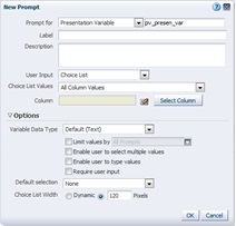
Its been long since I wrote any post related to OBIEE. It feels good to find some time to again share something with you guys. Everyone working on OBIEE would have read that OBIEE 11g has a capability to pass multiple values to presentation variable. To use this feature of OBIEE try to create variable dashboard prompt and link it to column whose values needs to be displayed in the prompt.


Tuesday, July 15, 2014

Essbase attribute dimension in OBIEE.

World is changing and becoming bigger and faster and so is the data and need to get useful information at seconds notice. Big organizations are demanding quality reports and decision making system which are even faster than Usain Bolt. Relational systems are good for transactional system but when it comes to DSS or OLAP system, multidimensional database, Hadoop are fast replacing relational databases. Essbase is becoming more and more prominent in datawarehousing and business intelligence world. Essbase's multidimensional structure and highly optimized server help in gaining that advantage over relational databases like Oracle and SQL server as far as performance in concerned.

Now with OBIEE also supporting essbase well, most of the business intelligence system are moving towards adopting essbase and OBIEE for datawarehousing and reporting system. As people having knowledge of OBIEE and essbase and its integration would say that it is very easy to expose any essbase cube in OBIEE , however sometimes there are a few things in essbase that gives pain while creating RPD. One of those is attribute dimension. Attribute dimension in an essbase cube is a separate helper dimension with other dimensions. While importing an essbase cube in OBIEE, all the dimensions would be imported using the outline present for an essbase cube. As you would guess, attribute dimension would also get imported as a separate dimension. However as attribute dimensions logically represent attributes of other dimension, it would make sense if the attributes are imported inside the base dimension itself. Consider a product dimension in an essbase cube having data for different products and its sales and cost data stored in the cube. These products has an attribute dimension called packagetype which gives what is the packaging type for a particular product. When using other reporting tools like smartview a person can select attribute value for which data needs to be analysed.

Attribute dimension selection in smartview

The above figure shows how we can select an attribute dinension value in smartview. However there can be a requirement to shows dimension members and corresponding attributes in a single place. OBIEE being a relational type reporting tool should do this be selecting the product member column exposed in OBIEE and corresponding attribute from the attribute dimension. However on the contrary when you do this you would get a report that would show you something like a cross product of all the members of product and packagetype dimension. This is the default behaviour of essbase as the MDX generated by default has a cross join keyword.

For example suppose the product dimension has 3 members as P1, P2 and P3 available and the attribute dimension has members as TinnedCan and CardBoardBox. Say that product P3 is only packaged as TinnedCan and others are packaged in CardBoardBox. So the logical report should show something like

Product                        PackageType
P1                                CardBoardBox
P2                                CardBoardBox
P3                                TinnedCan

However the result that would be displayed would be


Product                        PackageType
P1                                CardBoardBox
P1                                TinnedCan
P2                                CardBoardBox
P2                                TinnedCan 
P3                                CardBoardBox
P3                                TinnedCan

To resolve this issue we can create cube column in physical layer of RPD and move that column inside the base dimension, here inside product at correct generation level and change the column type to Attribute and in external name provide the external name or the name in essbase cube for that attribute dimension.

Attribute dimension column in OBIEE physical layer

Voila!!! This would resolve the issue of cross join and a user can easily generate dimension only reports in OBIEE with attributes as well. 

I guess this is all for today. We would meet and see another topic next time which can help us conquer the bigdata world. Till then Enjoy. :)

Monday, August 26, 2013

Aggregate Navigation in OBIEE


Starting from the last post, where we stopped about aggregation features in OBIEE. Today we will be discussing about aggregate navigation.To reap the benefit of pre aggregated fact tables OBIEE provides a way so that OBIEE automatically decides on itself which table to use for generating a report based on the aggregation level of the query.

To understand the concept of aggregate navigation, let us consider a situation where we have revenue calculated at detail day level (Revenue) and one aggregated at month level(Revenue Agg).  We would follow the below mentioned steps to activate aggregate navigation.

1.       First step is to import both the tables to physical layer of RPD.
2.       Now in the BMM layer, we would create a logical table Revenue.
3.       In the logical table “Revenue”, add a logical table source Revenue. This can be done by clicking on Revenue table in physical layer and dragging and dropping it on the “Revenue” logical table.
4.       On double clicking on LTS Revenue, we will see only Revenue LTS in the Map to these tables area showing that the columns of this logical table maps to only Revenue LTS.  Now drag the physical table Revenue_Agg from physical layer and drop it on logical table Revenue. After this we could see the LTS Revenue as well as Revenue_Agg in the logical table sources for logical table Revenue.
 
5.       Now as these tables in database are at different granular level hence we need to tell OBIEE that these tables are at different levels of granularity. To do this we first click on Revenue LTS and move to Content tab.

 
6.       Now if we do not specify any levels for different dimensions to which this table is related (Location, Product and Time here), then the default level of aggregation would be detail level for each dimensional hierarchy. However to specify different levels for time dimension on which Revenue tables are aggregated we need to specifically specify the level of aggregation in each LTS.

To do this in LTS Revenue content tab, we would specify detail level for time dimension.


Since we are not specifying any level for other dimensions, so the default now would be considered as total level for other dimensions. This is contrasting to when no level is specified for any of the dimensions in which case the default level is detail level.

So to get the correct functionality we would specify detail level for other dimensions too in Revenue LTS.

Now for the other LTS Revenue_Agg, specify period level as time dimension and detail level for other dimensions.


Now when a report is created with column from time dimension as period then Revenue_Agg is queried while if we have column which is lower than period level then Revenue table is queried.

Oracle analytics - Different pricing schems

OBIEE on premise Licensing: Component based licensing: The pricing is based on the user base or volume(COGS/revenue). It is a buy as ...